The Kalman Filter Explained

Q: What are the assumptions of the Kalman filter?

The standard Kalman Filter assumes linear system dynamics, Gaussian white process and measurement noise with known covariance matrices, and a Gaussian initial state estimate. When these hold, it is the optimal minimum mean-square error estimator.

Q: What happens when the Kalman filter assumptions are violated?

For non-linear dynamics, the Extended Kalman Filter (EKF) or Unscented Kalman Filter (UKF) can be used. For non-Gaussian or multi-modal distributions, Particle Filters (Sequential Monte Carlo) provide a more flexible alternative at greater computational cost.

Q: Is a Kalman filter a type of machine learning?

The Kalman Filter predates modern machine learning but can be viewed as exact Bayesian inference in a linear-Gaussian state-space model. It performs online learning of a latent variable model and is equivalent to Gaussian Process regression with a specific covariance structure.

A Step-by-Step Derivation

The Kalman Filter cycle: prediction step uses a physical model to advance the state estimate, then the update step corrects the prediction using measurements, producing a refined output estimate

The aim of this tutorial is to derive the filtering equations for the simplest Linear Dynamical System case — the Kalman Filter — outline the filter's implementation, do a similar thing for the smoothing equations and conclude with parameter learning in an LDS (calibrating the Kalman Filter).

What Is a Kalman Filter?

The Kalman Filter is an algorithm that estimates the hidden state of a linear dynamical system from a series of noisy measurements. Introduced by Rudolf Kalman in 1960, it is one of the most widely used algorithms in engineering and applied mathematics — powering everything from spacecraft navigation and GPS to financial time-series analysis and robotics.

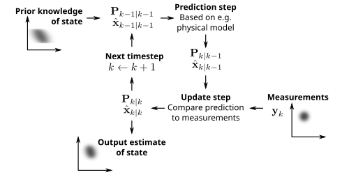
At its core, the filter maintains a belief about the current state of the system (represented as a Gaussian distribution) and refines that belief each time a new measurement arrives. The "predict" step projects the state forward using a physical or statistical model; the "update" step corrects the prediction using the observed data, weighting model and measurement according to their respective uncertainties.

Kalman Filter Applications and Practical Examples

The Kalman Filter is one of the most widely deployed algorithms in engineering. In GPS navigation, it fuses noisy satellite signals with inertial sensor data to produce smooth, accurate position estimates — every smartphone uses a variant of the Kalman Filter for location services. In autonomous vehicles, extended and unscented Kalman Filters track the position, velocity and heading of the car and surrounding objects from lidar, radar and camera measurements.

In aerospace, the Kalman Filter was originally developed for the Apollo navigation computer and remains central to spacecraft guidance and satellite orbit determination. In finance, it is used to estimate hidden states in time-series models — for example, extracting an unobservable "true" volatility or mean-reversion level from noisy market prices. In robotics, it underpins simultaneous localisation and mapping (SLAM), enabling robots to build a map of their environment while tracking their own position within it. In weather forecasting, variants of the Kalman Filter (ensemble Kalman Filters) assimilate observational data into numerical weather models.

Kalman Filter Tutorial: What You Will Learn

The Linear Dynamical System model
Deriving the Kalman filtering equations from first principles
The Kalman smoother
Parameter learning (EM algorithm for LDS)
Practical implementation guidance

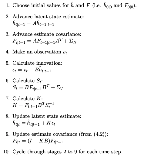
The filtering algorithm itself reduces to a ten-step cycle of prediction and correction:

The Kalman Filter algorithm: ten numbered steps from initialising state estimates and covariance, through prediction, innovation, Kalman gain computation, and state update, cycling for each time step

Filtering vs Smoothing

The tutorial distinguishes between filtering and smoothing. Filtering estimates the state at time t using only observations up to time t — this is the classic real-time Kalman Filter. Smoothing (also called the Rauch-Tung-Striebel smoother) estimates the state at time t using all observations, including future ones, giving a more accurate retrospective estimate. Both sets of equations are derived from first principles in the PDF.

Download the full tutorial (PDF)

Beyond the Standard Kalman Filter

The standard Kalman Filter assumes linear dynamics and Gaussian noise. When these assumptions are violated, several extensions exist. The Extended Kalman Filter (EKF) linearises non-linear dynamics around the current estimate using a first-order Taylor expansion. The Unscented Kalman Filter (UKF) uses a deterministic sampling technique (sigma points) to capture the mean and covariance of the state distribution more accurately through non-linear transformations, without requiring Jacobians. For highly non-linear or multi-modal problems, Particle Filters (Sequential Monte Carlo methods) represent the state distribution with a set of weighted samples, offering the most flexibility at greater computational cost.

Frequently Asked Questions about the Kalman Filter

What is a Kalman filter in simple terms?

A Kalman Filter is an algorithm that makes an educated guess about the state of a system (for example, the position and velocity of a moving object), then corrects that guess each time a new, noisy measurement arrives. It optimally balances how much to trust the prediction versus the measurement, based on how uncertain each one is. The result is a smooth, accurate estimate that is better than either the prediction or the measurement alone.

What is the difference between a Kalman filter and a Kalman smoother?

A Kalman Filter estimates the state at time t using only observations up to time t — it works in real time, making it suitable for online applications like navigation. A Kalman Smoother (such as the Rauch-Tung-Striebel smoother) estimates the state at time t using all observations, including future ones. This retrospective estimate is more accurate but requires the entire data sequence, making it suitable for offline analysis. Both are derived in the tutorial PDF.

What are the assumptions of the Kalman filter?

The standard Kalman Filter assumes: (1) the system dynamics are linear; (2) the process noise and measurement noise are Gaussian and white (uncorrelated over time); (3) the noise covariance matrices are known; and (4) the initial state estimate is Gaussian. When these assumptions hold, the Kalman Filter is the optimal estimator in the minimum mean-square error sense. When they are violated, extensions such as the Extended or Unscented Kalman Filter may be used.

What happens when the Kalman filter assumptions are violated?

If the dynamics are non-linear, the Extended Kalman Filter (EKF) or Unscented Kalman Filter (UKF) can be used. If the noise is non-Gaussian or the state distribution is multi-modal, Particle Filters (Sequential Monte Carlo) provide a more flexible alternative at greater computational cost. If the noise covariances are unknown, adaptive Kalman Filters estimate them online.

Where are Kalman filters used in practice?

Kalman Filters are used in GPS navigation, autonomous vehicles, spacecraft guidance, robotics (SLAM), weather forecasting, financial time-series analysis, signal processing, and control systems. Any application that involves estimating a hidden state from noisy sequential measurements is a candidate for Kalman filtering.

Is a Kalman filter a type of machine learning?

The Kalman Filter predates modern machine learning but is closely related. It can be viewed as exact Bayesian inference in a linear-Gaussian state-space model — a special case of a Hidden Markov Model with continuous states. In machine learning terminology, the Kalman Filter performs online learning of a latent variable model. It is also equivalent to Gaussian Process regression with a specific covariance structure defined by the state-space model.